Understanding Bayes’s Rule Through a Concrete Example

Bayes’s rule is a fundamental concept in probability theory, offering a robust framework for understanding conditional probabilities. This article delves into Bayes’s rule, illustrating its principles through a practical example and visualizations. The example is taken from Example 1.10.1 (Page 59 - 62) of the book An Introduction to Kolmogorov Complexity and Its Application, Fourth Edition, authored by Ming Li and Paul Vitányi.

Formal Statement of Bayes’s Rule

Bayes’s rule can be formally stated as follows:

$$ P(A | B) = \frac{P(B | A)P(A)}{P(B)} $$

where:

• $P(A | B)$ is the posterior probability of event $A$ given event $B$.
• $P(B | A)$ is the likelihood of event $B$ given event $A$.
• $P(A)$ is the prior probability of event $A$.
• $P(B)$ is the marginal probability of event $B$.

Illustrative Example: The Dice Urn

Consider an urn filled with dice, each having a unique probability $p$ of showing the number 6. The probability $p$ may differ from the 1 / 6 expected from a fair die. If we draw a die from the urn and roll it $n$ times, observing the number 6 $m$ times, we can use Bayes’s rule to understand the probabilities involved.

Prior Distribution

Let $P(X=p)$ represent the prior probability of drawing a die with probability $p$ of showing a 6. According to von Mises’s interpretation, the relative frequency of drawing a die with a specific $p$ converges to $P(X=p)$ over many draws.

Likelihood Function

The likelihood of observing $m$ outcomes of 6 in $n$ throws for a die with probability $p$ is given by the binomial distribution:

$$ P(Y=m | n, p) = \binom{n}{m} p ^ m(1 - p) ^ {n - m} $$

This represents the number of ways to choose $m$ successful outcomes from $n$ trials, multiplied by the likelihood of those successes and failures.

Posterior Distribution

Therefore, the probability of drawing a die with probability $p$ and subsequently observing $m$ outcomes of 6 in $n$ throws is the product $P(X=p)P(Y=m | n, p)$.

In this context, Bayes’s problem involves determining the probability of observing $m$ outcomes of 6 in $n$ throws due to a die with a specific probability $p$. The solution is given by the posterior or inferred probability distribution:

$$ P(X=p | n, m) = \frac{P(X=p)P(Y=m | n, p)}{\sum_{p} P(X=p)P(Y=m | n, p)} $$

Here, the denominator is the sum over all possible values of $p$, ensuring the probabilities sum to 1.

Experiments and Visualization

To understand these concepts better, let’s conduct a series of experiments and visualize the results.

Experiment 1: Uniform Prior

Let $p$ take values 0.1, 0.2, …, 0.9, each with equal probability $P(X=p) = 1 / 9$. We consider two cases: $n = 5, m = 3$ and $n = 500, m = 300$.

Case 1: $n=5, m=3$

Case 2: $n=500, m=300$

Experiment 2: Weighted Prior

Let the new prior distribution be $P(X=p) = i / 45, i = 1, …, 9$. We analyze the inferred probabilities for the same two cases.

Case 1: $n=5, m=3$

Case 2: $n=500, m=300$

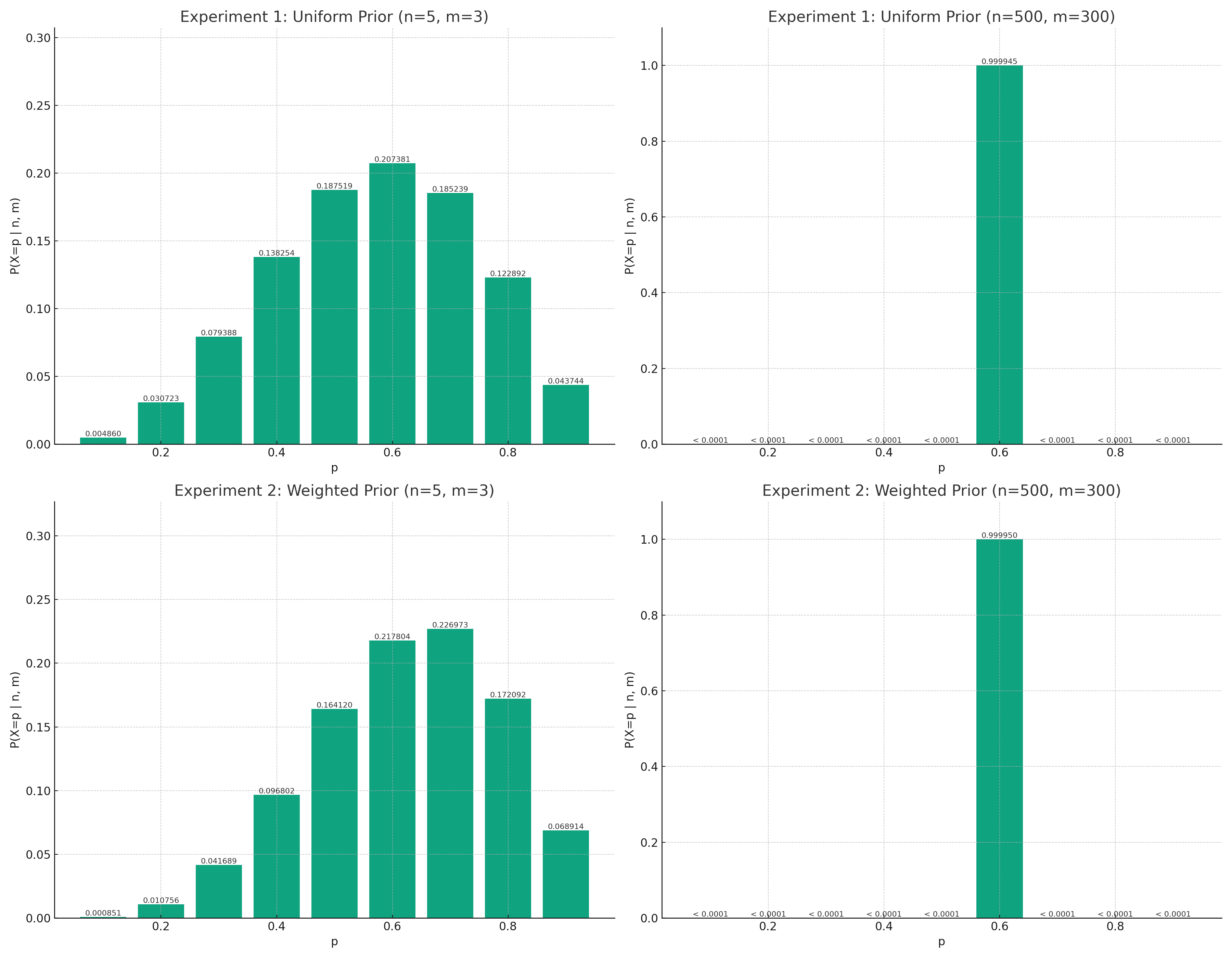
These experiments demonstrate that as the number of trials increases, the limiting value of the observed relative frequency of success approaches the true probability of success, regardless of the initial prior distribution. Bayes’s rule proves to be a powerful tool for making inferences based on a large number of observations. However, for small sequences of observations, knowledge of the initial probability is crucial for making justified inferences.

The codes for the experiments are generated by ChatGPT.

 1
 2
 3
 4
 5
 6
 7
 8
 9
10
11
12
13
14
15
16
17
18
19
20
21
22
23
24
25
26
27
28
29
30
31
32
33
34
35
36
37
38
39
40
41
42
43
44
45
46
47
48
49
50
51
52
53
54
55
56
57
58
59
60
61
62
63
64
65
66
67
68
69

import numpy as np
import matplotlib.pyplot as plt
from scipy.special import comb

# Define the binomial likelihood function


def binomial_likelihood(p, n, m):
    return comb(n, m) * (p**m) * ((1 - p)**(n - m))

# Calculate the posterior distribution


def posterior(p_values, prior, n, m):
    likelihoods = np.array([binomial_likelihood(p, n, m) for p in p_values])
    unnormalized_posterior = prior * likelihoods
    posterior = unnormalized_posterior / np.sum(unnormalized_posterior)
    return posterior


# Define p values and prior distributions
p_values = np.arange(0.1, 1, 0.1)
uniform_prior = np.array([1 / 9] * 9)
weighted_prior = np.array([i / 45 for i in range(1, 10)])

# Experiment 1: Uniform prior
posterior_uniform_5_3 = posterior(p_values, uniform_prior, 5, 3)
posterior_uniform_500_300 = posterior(p_values, uniform_prior, 500, 300)

# Experiment 2: Weighted prior
posterior_weighted_5_3 = posterior(p_values, weighted_prior, 5, 3)
posterior_weighted_500_300 = posterior(p_values, weighted_prior, 500, 300)


# Function to plot with more accurate numbers on top of the bars and save the image
def plot_with_accurate_labels_and_save(p_values, posteriors, titles, xlabel, ylabel, filename, figsize=(18, 14)):
    plt.figure(figsize=figsize)

    for i, (posterior, title) in enumerate(zip(posteriors, titles), 1):
        plt.subplot(2, 2, i)
        bars = plt.bar(p_values, posterior, width=0.08)
        plt.title(title)
        plt.xlabel(xlabel)
        plt.ylabel(ylabel)
        # Adjust y-limit to max value + 0.1 for better visualization
        plt.ylim(0, max(posterior) + 0.1)
        for bar, value in zip(bars, posterior):
            # More accurate label with 6 decimal places
            label = f"{value:.6f}" if value > 0.0001 else "< 0.0001"
            plt.text(bar.get_x() + bar.get_width() / 2, bar.get_height(), label,
                     ha='center', va='bottom', fontsize=8)

    plt.tight_layout()
    plt.savefig(f"/mnt/data/{filename}.png")
    plt.show()


# Call the function with all four experiments
plot_with_accurate_labels_and_save(
    p_values,
    [posterior_uniform_5_3, posterior_uniform_500_300,
        posterior_weighted_5_3, posterior_weighted_500_300],
    titles,
    'p',
    'P(X=p | n, m)',
    'bayes_experiments_accurate_labeled',
    figsize=(18, 14)
)

Conclusion

This approach quantifies the intuition that when the number of trials $n$ is small, the inferred distribution $P(X=p | n, m)$ heavily depends on the prior distribution $P(X=p)$. However, as $n$ increases, the inferred probability $P(X=p | n, m)$ increasingly concentrates around the empirical frequency $m / n = p$, regardless of the prior.