Purpose

• Dynamic Programming.
• Application of Sorting in Algorithm Design.

Problem Statement

Let’s schedule some jobs again! We have had a lab on job scheduling problem before and this time we consider jobs with weights.

The Lab is excerpted from Section 12.3 of Algorithm Design and Applications by Michael T. Goodrich and Roberto Tamassia. We also talked about weighted job scheduling in Kleinberg and Tardos. I will not repeat most of the contents in the books. I will just emphasis what I believe are the important aspects of the problem.

• Input: A list of jobs $L$. A job $i$ is specified by a triple: ($s_i$, $f_i$, $b_i$) meaning the starting time, finishing time, and the benefit of performing the job $i$.
• Output: A selected subset of the jobs, so that
  • No jobs in the subset are conflict with each other.
  • The sum of the benefits are maximized.

In the first book above, the problem is introduced via a vivid language and is called “telescope scheduling problem”. Below is an example taking out of the book.

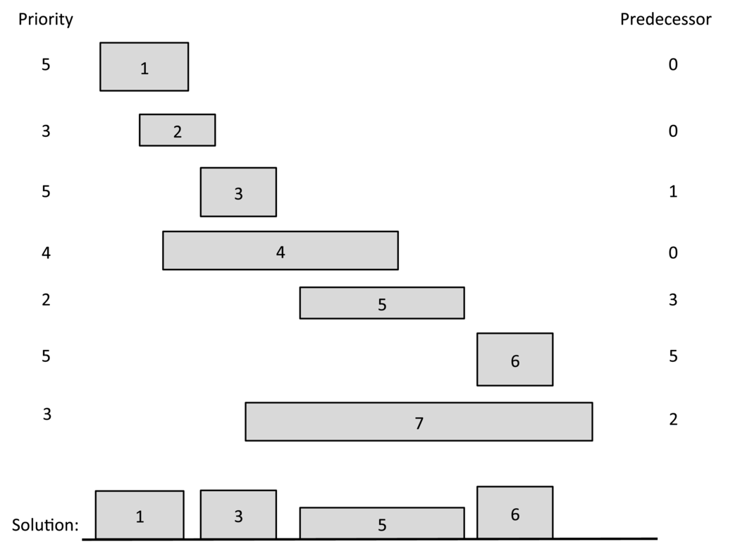Figure 1: The telescope scheduling problem. The left and right boundary of each rectangle represent the start and finish times for an observation request. The height of each rectangle represents its benefit. We list each request’s benefit on the left and its predecessor on the right. The requests are listed by increasing finish times. The optimal solution has total benefit 17 = 5+ 5+ 2+ 5.

Solution of The Problem

Dynamic Programming and Memoization

As we discussed in the lecture, we need the following notion.

We first assume $L$ is ordered by nondecreasing finish times.

\[ B_i = \text{the maximum benefit that can be achieved with the first $i$ request in $L$.} \] So, as a boundary condition, we get $B_0=0$.

We also define the predecessor, $pred(i)$, for each job $i$, to be the largest index $j$, such that $j$<$i$ and job $i$ and $j$ don’t conflict. If there is no such index, then define the predecessor of to be 0 (use -1 if index starting from 0).

The definition of the predecessor of each job lets us easily reason about the effect that including or not including a job, $i$, in a schedule that includes the first $i$ jobs in $L$. That is, in a schedule that achieves the optimal value, $B_i$, for $i>1$, either it includes the job $i$ or it doesn’t; hence, we can reason as follows:

• If the optimal schedule achieving the benefit $B_i$ includes job $i$, then $B_i= B_{pred(i)} + b_i$. If this were not the case, then we could get a better benefit by substituting the schedule achieving $B_{pred(i)}$ for the one we used from among those with indices at most $pred(i)$.
• On the other hand, if the optimal schedule achieving the benefit does not include job $i$ , then $B_{i-1}$. If this were not the case, then we could get a better benefit by using the schedule that achieves $B_{i-1}$.

Therefore, we can make the following recursive definition:

\[ B_i = \max\{B_{i-1}, B_{pred(i)}+ b_i\} \]

It is most efficient for us to use memoization when computing $B_i$. We use the arrays $B$ and $P$, and $B[i]$ and $P[i]$ for $B_i$ and $pred[i]$ respectively in the following code.

1
2
3

B[0]=0
for i=1  to n do:
    B[i]=max{B[i-1], B[P[i]]+ b_i}

We can see this algorithm runs in $O(n)$, where $n$ is the length of $L$. The bottleneck of the algorithm lies in the sorting of $L$, which costs $O(n\log(n))$. However, we still haven’t discuss how to compute $P[i]$ or $pred(i)$.

How to Compute $pred(i)$

Naive Linear Search

If you do a Google search, you will easily find solutions using naive way to solve the problem.

For example, this one’s Python implementation

 1
 2
 3
 4
 5
 6
 7
 8
 9
10

# Find the latest job (in sorted array) that
# doesn't conflict with the job[i]. If there
# is no compatible job, then it returns -1
def latestNonConflict(arr, i):

    for j in range(i - 1, -1, -1):
        if arr[j].finish <= arr[i - 1].start:
            return j

    return -1

does a linear search for each job $i$, and you need to do it for every $i$. So the complexity of calculating $P[]$ in this way is $O(n^2)$.

Binary Search

You can improve the above process by using binary search. See this link for the full solution. Basically, since the jobs already sorted by finish time, you just need to binary search for the first job so that its finish time is earlier than the target job’s start time.

 1
 2
 3
 4
 5
 6
 7
 8
 9
10
11
12
13
14
15
16
17
18
19
20
21
22
23

# A Binary Search based function to find the latest job
# (before current job) that doesn't conflict with current
# job.  "index" is index of the current job.  This function
# returns -1 if all jobs before index conflict with it.
# The array jobs[] is sorted in increasing order of finish
# time.
def binarySearch(job, start_index):

    # Initialize 'lo' and 'hi' for Binary Search
    lo = 0
    hi = start_index - 1

    # Perform binary Search iteratively
    while lo <= hi:
        mid = (lo + hi) // 2
        if job[mid].finish <= job[start_index].start:
            if job[mid + 1].finish <= job[start_index].start:
                lo = mid + 1
            else:
                return mid
        else:
            hi = mid - 1
    return -1

This method takes $O(\log(n))$ time to compute $pred(i)$ for each $i$. So in total it costs $O(n\log(n))$ time.

Some implementations use in Python use bisect module for binary search.

An $O(n)$ Algorithm Once and For All

The previous solutions compute $pred(i)$ for each $i$ separately. We now introduce a method to compute $pred(i)$ for all $i$ all at once.

In the Algorithms and Their Applications, a proposed way to do it

In particular, given a listing of $L$ ordered by finish times and another listing, $L'$, ordered by start times, then a merging of these two lists, as in the merge-sort algorithm, gives us what we want.

The predecessor of request $i$ is literally the index of the predecessor in $L$ of the value, $s_i$, in $L'$.

1. We have job $i$’s start time, $s_i$, in our hand.
2. Look at the merged list of $L$ and $L’$, find out $s_i$’s predecessor (but it need to be a finish time $e$). (If its predecessor is a start time, keep looking until you find an end time).
3. Report the index, $j$, of the finish time. (Which job it is coming form.) That is, set pred(i)=j.

In implementation, I modified the above process slightly.

1. I don’t really store the merged list to save space. But I do write out the merging process.
2. The two cursors in the merging algorithm will keep a record on the index of the end time naturally. So I don’t need to “keep looking until I find the end time”.
3. But I need to maintain a map between the start time and its original index before sorting. Note that I originally indexed the jobs by the end time.

Index the job by end time.

1
2
3
4

# zip the three lists
jobs = sorted([(e, s, p) 
       for e, s, p 
       in zip(endTime, startTime, profit)])

Bind the start time and the job index.

1
2
3
4
5

# map between the start time and its original job index.
jobs_by_start = sorted([
         (s, index)
        for index, (e, s, p) 
        in enumerate(jobs)])

The merging process. Computing pred() for all jobs once and for all.

 1
 2
 3
 4
 5
 6
 7
 8
 9
10
11
12
13

# ends: "jobs" as in the above
# starts: "jobs_by_start" as in the above
# P: the pred() function, stored in a list. 
def merge(self, ends, starts, P):
        j = 0 # cursor for end time 
        i = 0 # cursor for start time
        while j < len(ends) and i < len(starts):
            if ends[j][0] <= starts[i][0]:
                j += 1
            else:
                # we might want to do i-1, if we want things starting from 0
                P[starts[i][1]] = j - 1
                i += 1

Note that the algorithm does not work theoretically better than the previous binary searching algorithm, since it require the input to be sorted.

The full implementation can be found here. I changed some variables’ name for consistency with the current blog piece.