

The Entropy of Three Outcomes, in 3D
Xiang Huang / 2026-09-24
A coin has one free parameter, so its entropy is a curve. A three-sided die has two, so its entropy is a surface. Here is that surface, and you can turn it around.
For a distribution $(p_1, p_2, p_3)$ with $p_1 + p_2 + p_3 = 1$, the Shannon entropy is $$ H(p_1, p_2, p_3) = -\sum_{i=1}^{3} p_i \log_2 p_i . $$ The domain is the probability simplex, a triangle, and the graph of $H$ over it is a dome. Drag to rotate it, scroll or pinch to zoom, and hover or tap to read off a distribution.
Laying the simplex flat
Write $(x, y, z)$ for $(p_1, p_2, p_3)$. The quickest way to plot is to eliminate $z$ and draw $H(x, y, 1 - x - y)$ over the triangle $x, y \ge 0$, $x + y \le 1$ in the $xy$-plane. But that triangle is not the simplex. It is the simplex’s shadow on the $xy$-plane, a right isosceles triangle, so the picture comes out lopsided. The three outcomes play identical roles in $H$, yet they no longer look alike.
The fix is to put coordinates on the plane $x + y + z = 1$ itself. Call the corners $A = (0, 0, 1)$, $B = (1, 0, 0)$ and $C = (0, 1, 0)$. Take $B$ as the new origin, the edge $BC$ as the $u$-axis, and the line in plane $ABC$ through $B$ perpendicular to $BC$ as the $v$-axis. Given a point $P = (u, v)$ in the plane, we want its original coordinates $(x, y, z)$. Everything follows from one angle, the angle between plane $ABC$ and the $xy$-plane. Figure 1 walks through the construction step by step. Rotate it to see it from any side.
Figure 1. The plane $x + y + z = 1$ (blue) and its shadow on the $xy$-plane (beige). Use the buttons to step through the construction and the sliders to move $P$. Segments with the same color play the same role in the two similar triangles. Open it full-page.
Step 1: the angle between the planes. Let $M$ be the midpoint of $BC$. In the equilateral triangle $ABC$ the median $AM$ is perpendicular to $BC$, and in the right isosceles triangle $OBC$ so is $OM$. So $\theta = \angle AMO$ is the angle between the two planes. It sits in the right triangle $AOM$, with $$ AO = 1, \qquad OM = \frac{\sqrt{2}}{2}, \qquad AM = \frac{\sqrt{6}}{2}. $$
Step 2: lift $P$. Let $F$ be the foot of the perpendicular from $P$ to $BC$, so $PF = v$ and $BF = u$. Let $Q$ be the shadow of $P$ on the $xy$-plane, so $PQ = z$. Write $w = QF$ for the length of the shadow of $PF$. The line $BC$ is perpendicular to both $PF$ and the vertical $PQ$, so it is perpendicular to the whole plane $PQF$. In particular $QF \perp BC$, so the angle at $F$ is again $\theta$, and triangle $PQF$ is similar to triangle $AOM$: $$ z = v \cdot \frac{AO}{AM} = \frac{2v}{\sqrt{6}}, \qquad w = v \cdot \frac{OM}{AM} = \frac{v}{\sqrt{3}}. $$
Step 3: the shadow. Now work in the $xy$-plane, where triangle $OBC$ has $45^\circ$ angles at $B$ and $C$. Let $G$ be the point on $BC$ with the same $x$-coordinate as $Q$. Walk along $BC$ from $B$ to $C$:
- $BF = u$;
- $FG = w$, since $QFG$ is an isosceles right triangle;
- $GC = \sqrt{2}\,x$, since $G = (x, 1 - x)$ is at distance $x$ from the $y$-axis.
The three pieces make up $BC = \sqrt{2}$, so $$ u + w + \sqrt{2}\,x = \sqrt{2} \quad\Longrightarrow\quad x = \frac{\sqrt{2} - u - v/\sqrt{3}}{\sqrt{2}}. $$
Step 4: $y$. $Q$ is at distance $w$ from the line $x + y = 1$, so $x + y = 1 - \sqrt{2}\,w$. That gives $$ y = 1 - x - \frac{\sqrt{2}\,v}{\sqrt{3}}. $$ As a check, $z = 2v/\sqrt{6} = \sqrt{2}\,w$, so $x + y + z = 1$.
Altogether,
$$
x = \frac{\sqrt{2} - u - v/\sqrt{3}}{\sqrt{2}}, \qquad
y = 1 - x - \frac{\sqrt{2}\,v}{\sqrt{3}}, \qquad
z = \frac{2v}{\sqrt{6}}.
$$
The triangle itself is $v \ge 0$ together with
$$
v \le \sqrt{3}\,u \quad \text{for } 0 \le u \le \tfrac{\sqrt{2}}{2}, \qquad
v \le \sqrt{6} - \sqrt{3}\,u \quad \text{for } \tfrac{\sqrt{2}}{2} \le u \le \sqrt{2}.
$$
These two conditions are the sides $BA$ and $CA$. These are exactly the formulas and the RegionFunction in my original Mathematica notebook. The map $(u, v) \mapsto (x, y, z)$ is an isometry, since it sends one equilateral triangle of side $\sqrt{2}$ onto another. So the plot shows the simplex at its true shape.
Another way to see it
There is also a shortcut that never leaves the plane. Each of $x$, $y$, $z$ is an affine function on the triangle. It is $1$ at its own corner and $0$ along the opposite side, since that whole side lies in the plane where the coordinate vanishes. An affine function that vanishes along a line is proportional to the distance from that line. So each coordinate is the distance from $P$ to the opposite side divided by the altitude $h = \sqrt{6}/2$: $$ x = \frac{d_B}{h}, \qquad y = \frac{d_C}{h}, \qquad z = \frac{d_A}{h}. $$ As a bonus, $x + y + z = 1$ becomes $d_A + d_B + d_C = h$. This is Viviani’s theorem: from any point inside an equilateral triangle, the distances to the three sides add up to the altitude.
| corner | distance to opposite side | coordinate |
|---|---|---|
| B | ||
| C | ||
| A | ||
| sum |
In Figure 2 the three sides lie on the lines $v = 0$ (side $BC$), $v = \sqrt{3}\,u$ (side $BA$) and $\sqrt{3}\,u + v = \sqrt{6}$ (side $CA$). The point-to-line distance formula gives $$ d_A = v, \qquad d_C = \frac{\sqrt{3}\,u - v}{2}, \qquad d_B = \frac{\sqrt{6} - \sqrt{3}\,u - v}{2}, $$ and dividing by $h$, $$ x = \frac{\sqrt{6} - \sqrt{3}\,u - v}{\sqrt{6}}, \qquad y = \frac{\sqrt{3}\,u - v}{\sqrt{6}}, \qquad z = \frac{2v}{\sqrt{6}}. $$ This is the same map as before, written symmetrically. The interactive plot at the top uses the same idea in the forward direction. It places the corners $V_1, V_2, V_3$ of an equilateral triangle and sends $(p_1, p_2, p_3) \mapsto p_1 V_1 + p_2 V_2 + p_3 V_3$.
What to look for
The corners are at zero. A distribution with all its mass on one outcome has no uncertainty.
The edges are the binary entropy curve. On the edge $p_3 = 0$ we are back to a coin, and $$ H(p, 1-p, 0) = h(p) = -p\log_2 p - (1-p)\log_2(1-p). $$ The orange curves in the plot are three copies of $h$. Each peaks at 1 bit at the midpoint of its edge.
The top is at $\log_2 3$. By Jensen’s inequality applied to the concave function $\log_2$, $$ H = \sum_i p_i \log_2 \frac{1}{p_i} \le \log_2 \sum_i p_i \cdot \frac{1}{p_i} = \log_2 3 \approx 1.585, $$ with equality exactly at the uniform distribution $(\tfrac13, \tfrac13, \tfrac13)$.
The contours are convex. $H$ is concave, so each super-level set $\{H \ge c\}$ is convex. The contour lines are nested convex curves around the peak. The heavy contour at $H = 1$ is a nice one: it touches the boundary at exactly the three edge midpoints, because 1 bit is the most any single edge can reach.
The walls are vertical. Start on the edge $p_3 = 0$ and move a small amount $t$ inward, taking $t/2$ from each of $p_1$ and $p_2$. The first-order change in $H$ is $$ t\left(\tfrac12\log_2 p_1 + \tfrac12\log_2 p_2 - \log_2 t\right) + O(t), $$ and the $-t\log_2 t$ term dominates. The slope $\log_2(1/t)$ blows up as $t \to 0$. Adding even a tiny chance of a third outcome raises the uncertainty very fast. In the side view the surface meets the boundary with a vertical tangent.
A printed copy
The surface also exists as a physical object. I 3D-printed it, and it stands on its three corners, the pure distributions where $H = 0$.
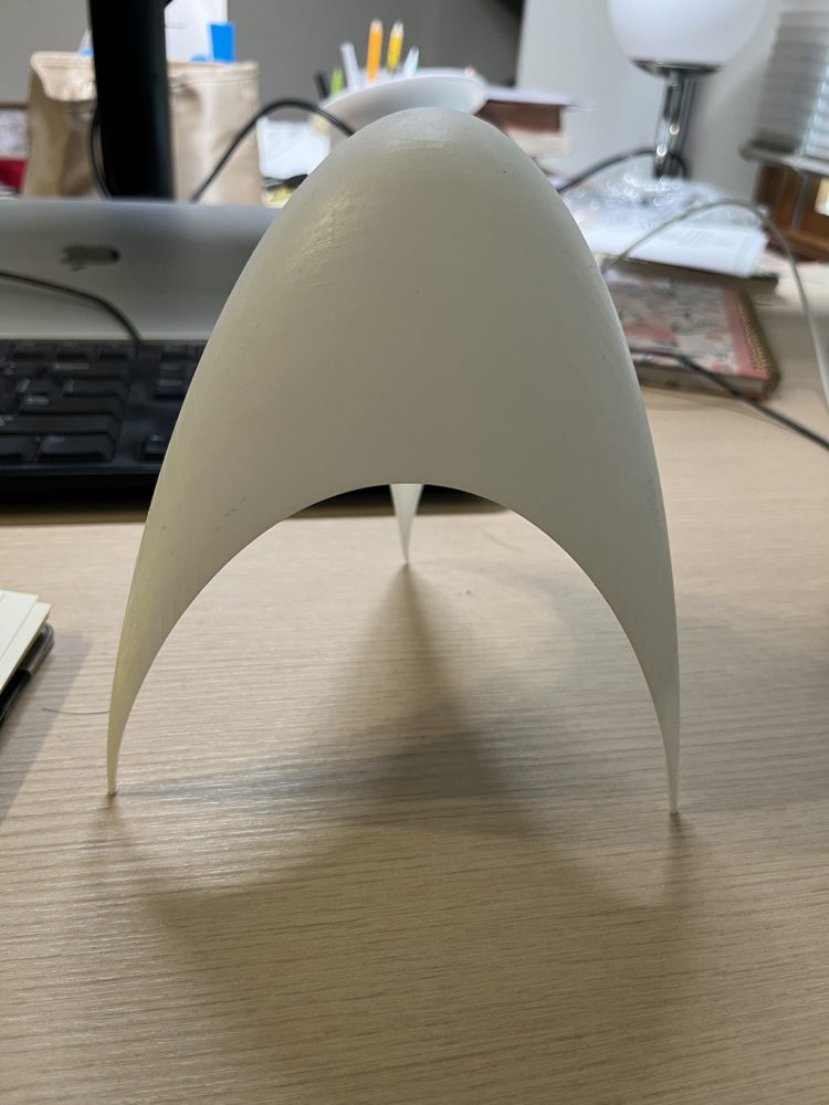
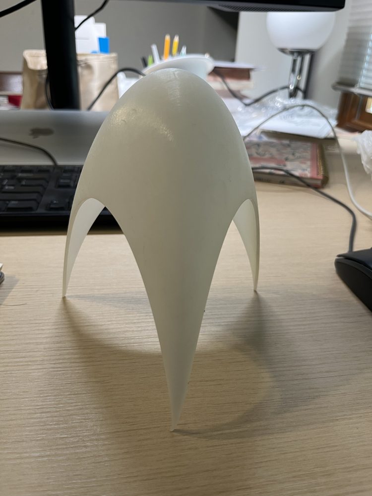
The needle-sharp legs are the vertical walls from above. Along an edge, near a corner, the height is $h(p) \approx p \log_2 (1/p)$, whose slope blows up as $p \to 0$. So each edge curve comes down to the table vertically, and the three legs taper to points.
Print your own. Download entropy-surface.stl (binary STL, 4.9 MB). It is generated directly from the formula, so the heights are exact everywhere, including along all three edges. It is a closed shell in millimetres: 100 mm along each edge of the base, 112 mm tall, with a 1.2 mm wall that tapers to a point at the three tips. Scale it freely in your slicer. The generator script can make other sizes and wall thicknesses.
Why redraw it
I first drew this in Mathematica with ParametricPlot3D over a rectangle in $(u,v)$, cut down to the triangle with RegionFunction. The picture was never quite right. Clipping a square grid leaves a ragged edge, the vertical walls come out faceted, and a rainbow color map hides where the surface is actually high.
The version above uses a triangular grid laid out in the $p_i$ themselves, so the boundary is exact. Color, contours and lighting are computed per pixel from the formula and its exact gradient, so the steep walls stay smooth. Color runs from dark (certain) to light (uncertain). The faint grid marks $p_i = 0.1, 0.2, \ldots$, and the floor repeats the contours as a flat ternary diagram.
The code is on GitHub.